`rspsp`: Spatial Spectral Analysis Toolkit • rspsp

rspsp contains tools for analyzing spatial lattice data. Its main features include:

Samplers for random data
Diagnostic tools for assessing the spectrum
Test statistics for modeling assumptions and comparing spectra

Generating Random Data

One of the easiest ways of fetching practice data for our tool is to generate new synthetic data. We offer two different spatial processes and one correlated extension:

To generate a sample, simply generate coefficients using one of our utils (MA_coef_all(), MA_coef_row(), MA_coef_col()) and then use the sampler. For details on the usage of other samplers you can see Reference.:

# generate new coefficient matrix for 
K0 <- MA_coef_all(.5)

x <- gridMA(75, 75, K0)

image(x)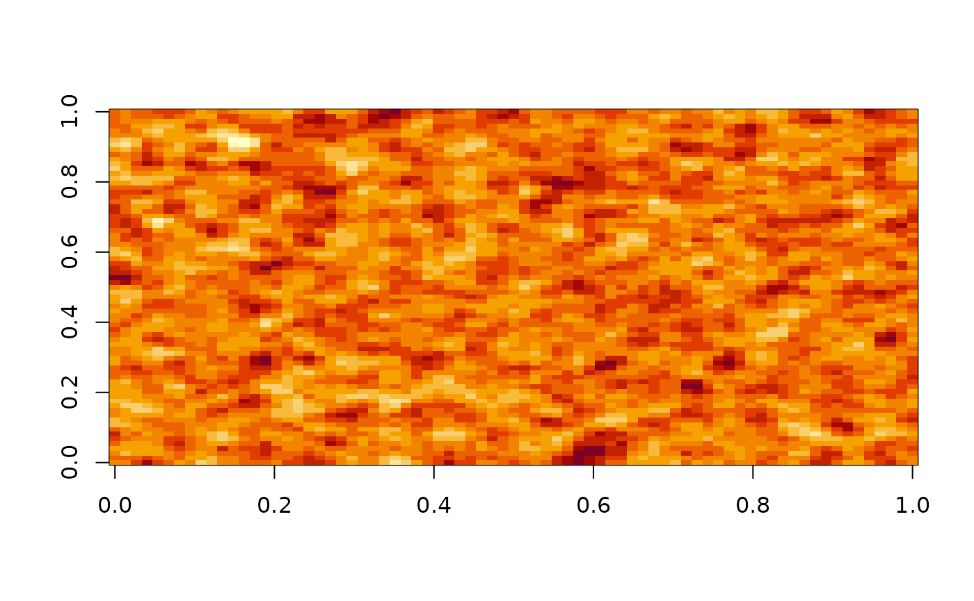

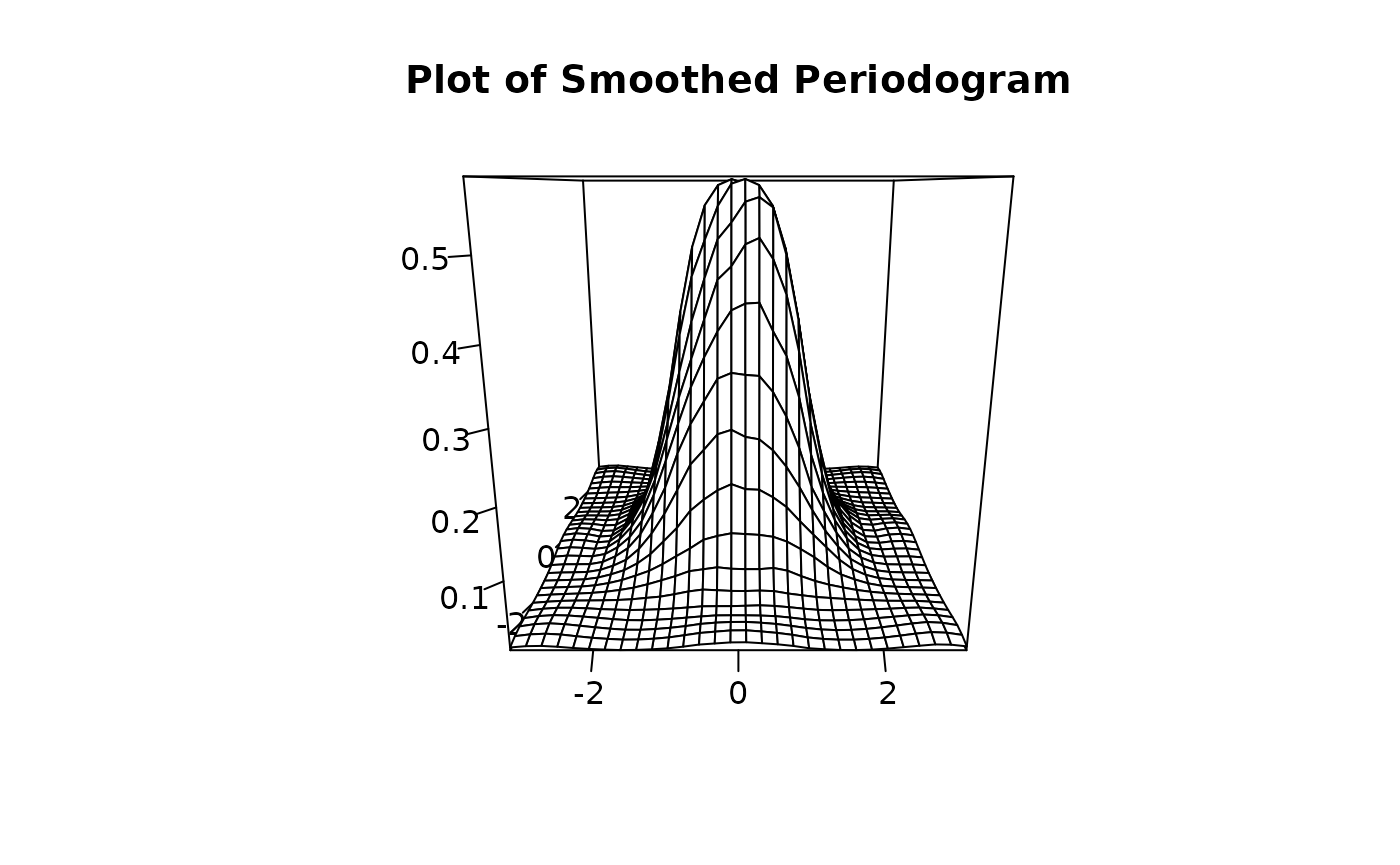
Inspecting the Periodogram and Spectral Density

Before testing your sample you can inspect the spectral properties with the I() function:

image(I(x))

To inspect the spectral density estimate use I_smooth() we also offer a plot generic for the returned object:

I_x_smooth <- I_smooth(I(x))

plot(I_x_smooth)

Testing for Equal Spectra

Test for equal spectra by either using by one of test.periodo() or test.spectral().

y <- gridMA(75, 75, K0)

# apply periodogram based test Scaccia and Marin (2005)
summary(test.periodo(x, y, .05))
#> Periodogram Test for equality Hypothesis. 
#> =========================================
#> alpha: 0.05 
#> 
#> 
#> Results 
#> -----------------------------------------
#> Tn: -1.444126 
#> p: 0.9256483 
#> Decision: Accepted H0

# apply randomized test after Jentsch and Pauly (2015)
res <- test.spectral(x, y, 300, .05)
summary(res)
#> Resampling Test for equality Hypothesis. 
#> =========================================
#> Resampling iterations: 300 
#> alpha: 0.05 
#> used kernel-bandwith: 
#>  h1: 0.05624503 h2: 0.05624503
#> 
#> Results 
#> -----------------------------------------
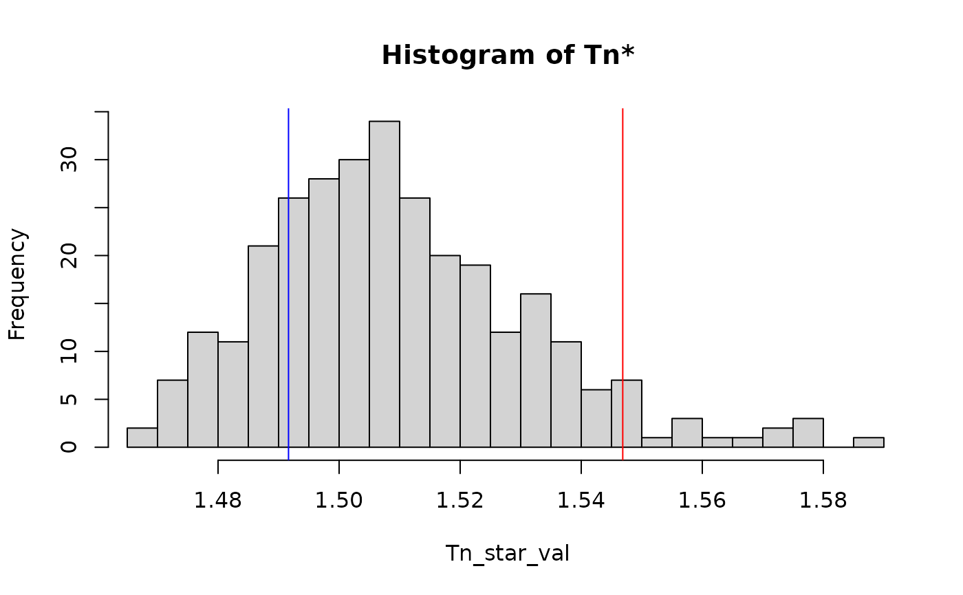
#> Tn: 27.18329 
#> p: 0.7666667 
#> Decision: Accepted H0

You can also visualize the distribution of the randomized samples against the L_2 type test T_n (see test_spectral() for more detail):

plot(res)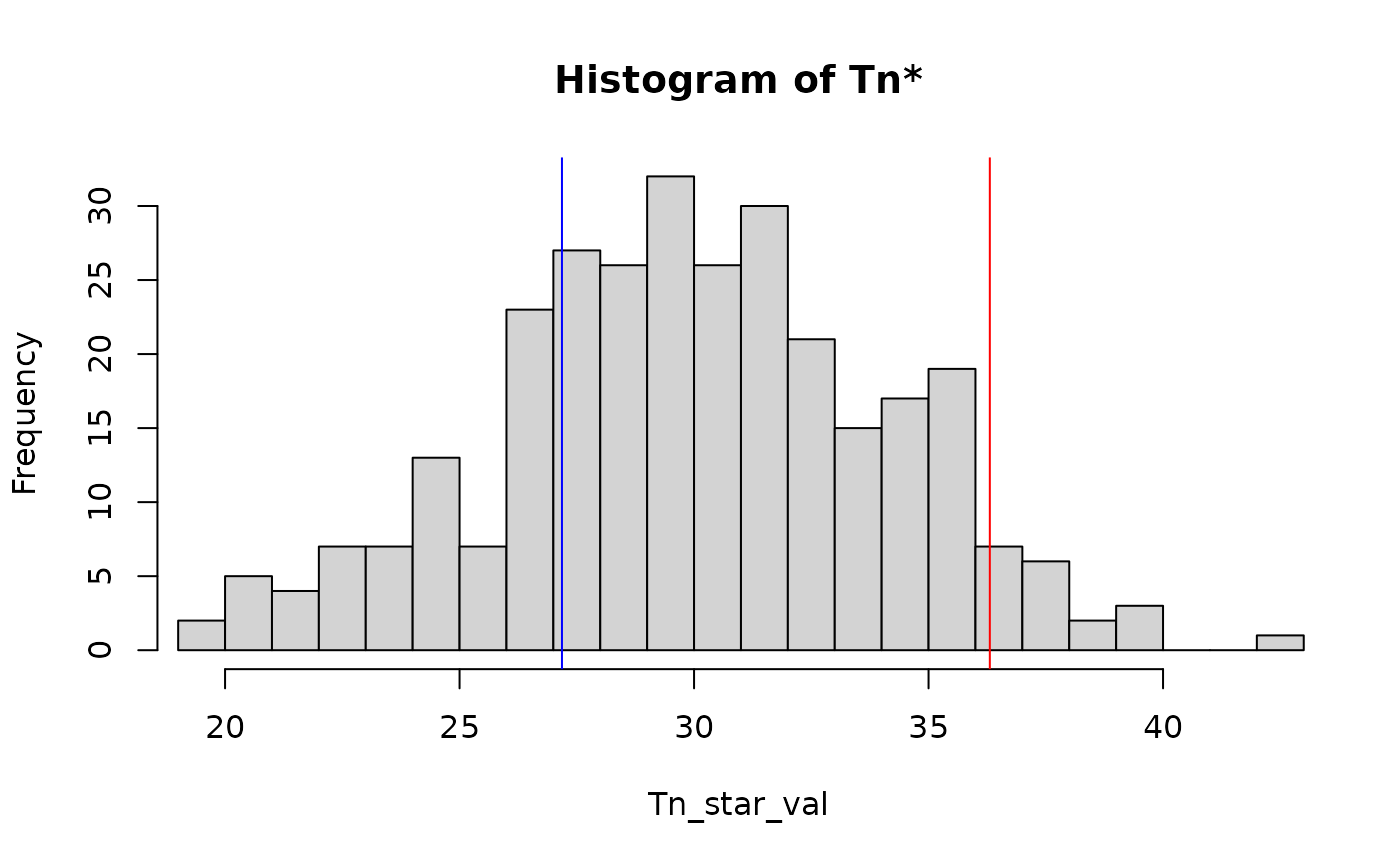

Testing for Isotropy

test.spectral() is applicable to other hypothesis for modelling assumptions. If you want to test for weak isotropy simply set hypothesis="isotropy"

# make sure to pass NULL for y
res <- test.spectral(x, NULL, 300, .05, hypothesis="isotropy")

summary(res)
#> Resampling Test for isotropy Hypothesis. 
#> =========================================
#> Resampling iterations: 300 
#> alpha: 0.05 
#> used kernel-bandwith: 
#>  h1: 0.05624503 h2: 0.05624503
#> 
#> Results 
#> -----------------------------------------
#> Tn: 18.77008 
#> p: 0.9266667 
#> Decision: Accepted H0
plot(res)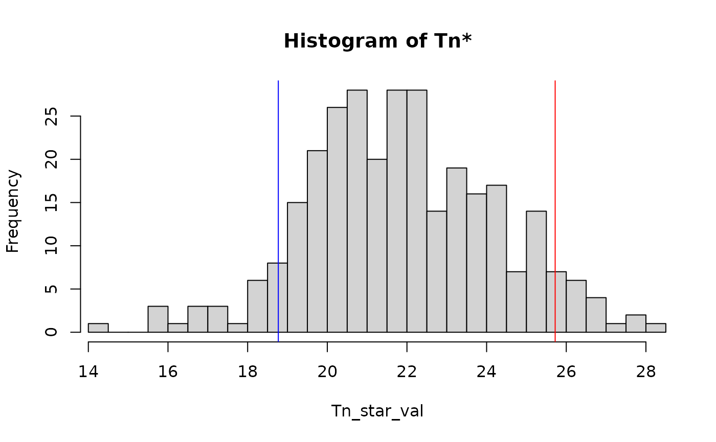

If we would now consider a non-isotropic process:

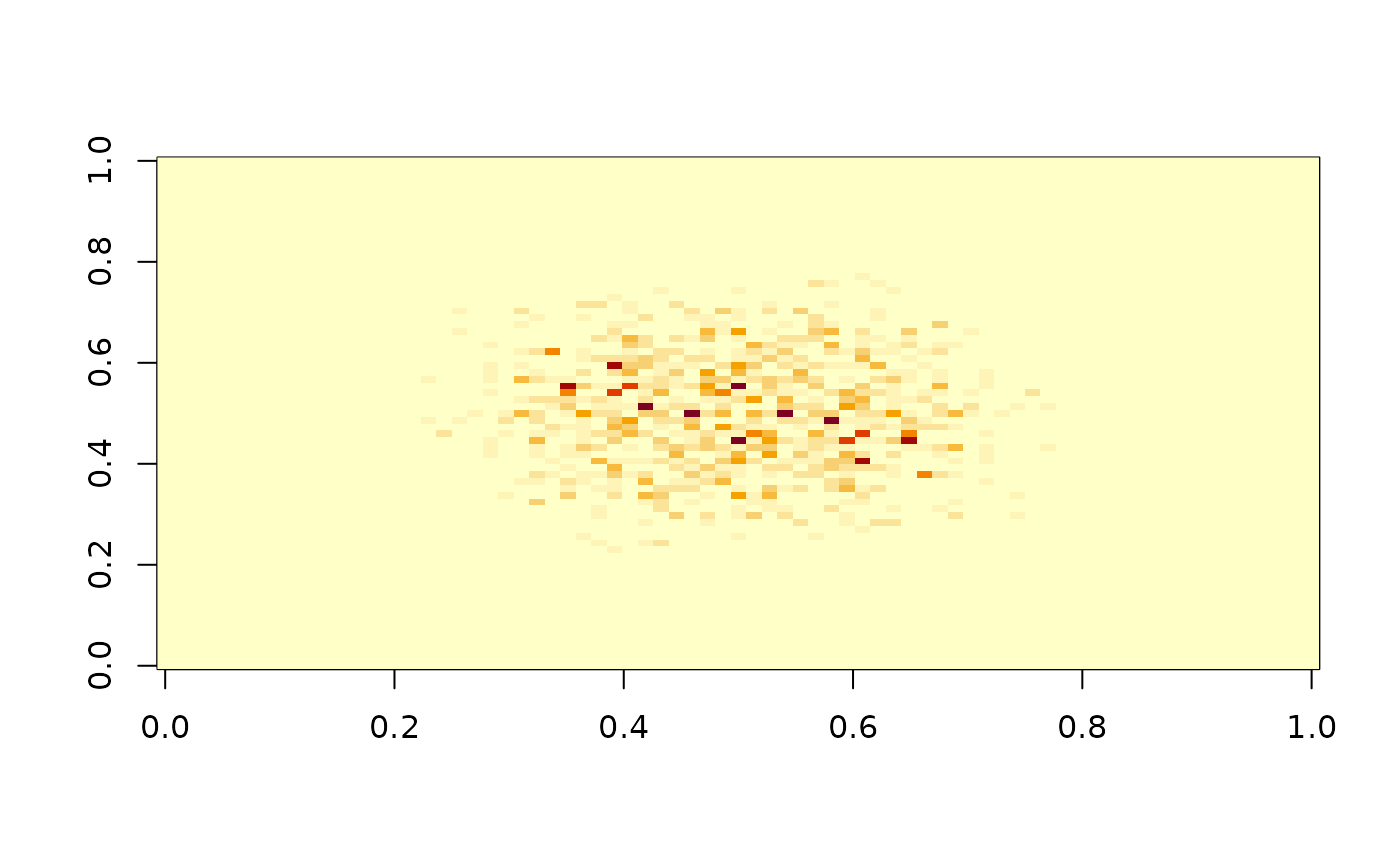
x <- gridMA(50, 50, MA_coef_row(.7))
image(I(x))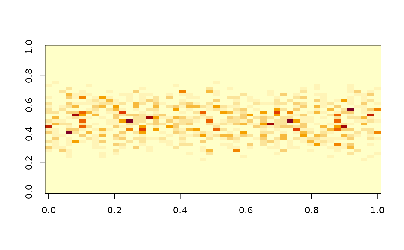

…the test will reject:

res <- test.spectral(x, NULL, 300, .05, hypothesis="isotropy")
summary(res)
#> Resampling Test for isotropy Hypothesis. 
#> =========================================
#> Resampling iterations: 300 
#> alpha: 0.05 
#> used kernel-bandwith: 
#>  h1: 0.07369985 h2: 0.07369985
#> 
#> Results 
#> -----------------------------------------
#> Tn: 15.71547 
#> p: 0 
#> Decision: Rejected H0

plot(res)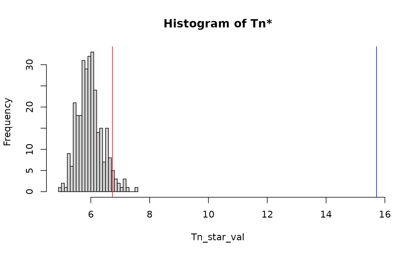

you can also test for weak stationarity using hypothesis=stationary

h <- length(x)^(-.2)
res <- test.spectral(x, NULL, 300, .05, hypothesis="stationary", h1=h, h2=h)

summary(res)
#> Resampling Test for stationary Hypothesis. 
#> =========================================
#> Resampling iterations: 300 
#> alpha: 0.05 
#> used kernel-bandwith: 
#>  h1: 0.2091279 h2: 0.2091279
#> 
#> Results 
#> -----------------------------------------
#> Tn: 1.491642 
#> p: 0.8066667 
#> Decision: Accepted H0
plot(res)